Training a Model on 100 Million Ratings with Spark on a Mac M1

Is it possible to train a model on 100 million rows using nothing more than a common laptop?

I've been refreshing Spark lately and wanted to give it a try on a dataset I wouldn't be able to deal with using non-big data tools such as Pandas and Numpy. I came across the dataset and the Netflix challenge it originates from some time ago, but have never really had any reason to work on it. Until now. The complete notebook can be found on GitHub here.

The dataset is open source and available on Kaggle through this link.

Prepare, Merge and Convert the Data to Parquet Format

The data comes ill-suited for analysis and needs to be prepared in a couple of steps before we can proceed. The following code snippet loads the original .txt files, extracts the movieID, which is stored in a way that makes further analysis difficult, adds a column for corresponding before storing each file in .csv format. The script may take some time as we are processing over 100 million rows.

Next, we will add the release year for each movie as the YearOfRelease column to the data by joining it with the movie_titles.csv file. Lastly, we convert the resulting CSV files to Parquet format for compuational benefits later on.

To make sure each column is of expected data type, we create a schema for each. The schema is then used when loading the data as shown below.

Let's now join the two DataFrames keeping only the columns we are interested in - which are all columns in the ratings DataFrame, but only YearOfRelease in movie_titles. We join them on the common column MovieID. In order to select only the columns we're interested in, we create an alias for each of the DataFrames. While we're on to it, we can also shuffle the data so the ordering (e.g. most recent movies at the top) doesn't affect the analysis. The code for that looks as follows.

This is how the resulting data looks like:

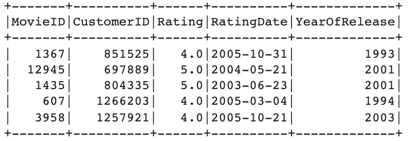
Lastly, we convert and store the data locally in Parquet format. This results in a significantly more efficient data processing while also taking up less space on the disk. The disadvantage is that it's hard for the human eye to interpret and understand these files as they are stored in binary format. The CSV files we've been working with up to now can easily be opened up and inspected with common tools such as Excel.

Initial Exploratory Data Analysis

Now when the data has gone through some initial preparation and convertion we can take a closer look at it. Start by initiating a SparkContext and SparkSession. To deal with potential memory issues during later model training on the full dataset, the following settings in the spark-default.conf file will help prevent those.

Once the data is loaded, we can display som descriptive statistics to get a better general understanding of it.

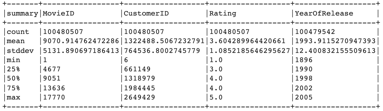
We can verify that there are around 100 million ratings (100,480,507 to be precise). Additionally, we make the following observations:

• There are 17,770 unique movies.
• There are 480,189 unique customers (or users). Note that this is not depicted in the summary above - see the notebook for details.
• Movie ratings are provided in a scale between 1 and 5. The average movie rating among all movies is quite positive at 3.6.
• The oldest movie in the dataset was released in 1896, while the most recent is from 2005.
• There are 965 missing values in the YearOfRelease column.

While we will do a more thorough visulisation of the dataset efter engineering more features (to keep everything in one place and to facilitate for the purpose of this writing), we can already now remove missing values. We can then confirm that no missing values are present by selecting only rows with missing values. If the output is empty, we're good to go.

The result of above yields the following.

Confirmed - there are no NULL values left. We can move on to creating some new feaures.

Feature Engineering

We will do some simple feature engineering by extracting year and month from the RatingDate column as well as calculating the difference in years between that column and the YearOfRelease column. Perhaps knowing when the rating was given and its relation to the release date might better help us determine what rating was given by a specific user. We should also make sure to convert the columns to adequate data types using the .cast() method.

Engineering the difference, Diff_RatingRelease, is the trickiest and needs some extra workarounds. What we do is that we calculate the difference in years between the release and rating year before dividing by 365.25 to convert it into days.

Additionally, we can bin the Diff_RatingRelease column into Diff_binned to have fewer categories to deal with. This can speed up model training as well. We could experiment by binning in several different ways before training and evaluating a model to find the most suitable bins for the problem. For the purpose of this notebook, we will take a shortcut and bin in the following way:

Values	Bin
Negative	-1
0 - 4.99	0, 1, 2, 3, 4 and 5, respectively
5 - 9.99	5
10 - 49.99	10
50 and above	50

The logic for that is coded in the bin_diff() function below.

Moreover, we have some categorical variables that should be treated before moving forward. These are the nominal variables MovieID and CustomerID. Under current rank order representation, the model may learn that, for example, the customer with CustomerID 1488844 is larger/bigger/worth more than the customer with CustomerID 822109 (simply because its CustomerID is higher). Such bias is misleading and we need to address that. There are several options we can take, such as one-hot encoding and bin-counting, but we will go with hashing as it's more straight forward and offers significant computational advantages when we have 480k unique customers. Spark's FeatureHasher is well suited for this.

We leave the ordinal variables YearOfRelease, RatingYear and RatingsMonth as they are since they are sensitive to rank order (i.e. it makes sense to say that release year 2000 is more recent, or higher, than 1995).

After applying above steps, we end up with the following data:

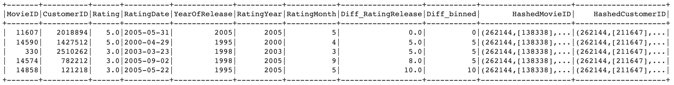
Let's keep the target variable Rating as a float. This allows us to approach it as a regression rather than as a classification problem, with the advantage of providing us with the size of the error on each prediction. With a classification approach, predicting a rating of 4 on a movie, which actually got a 3, is equally bad as predicting it as receiving a 1. That doesn't seem reasonable, and a regression approach would be able to better deal with this.

Data Visualisation

Next, let's plot the count for each categorical column to get an estimate of their distribution per category. The MovieID and CustomerID columns are truncated due to their large numbers and only display the lowest five (which each has count=1) and highest 100 counts. We also sort these columns on their counts to facilitate interpretation. The hashed columns are excluded from the visualisation as they are hard to interpret for the human eye anyway.

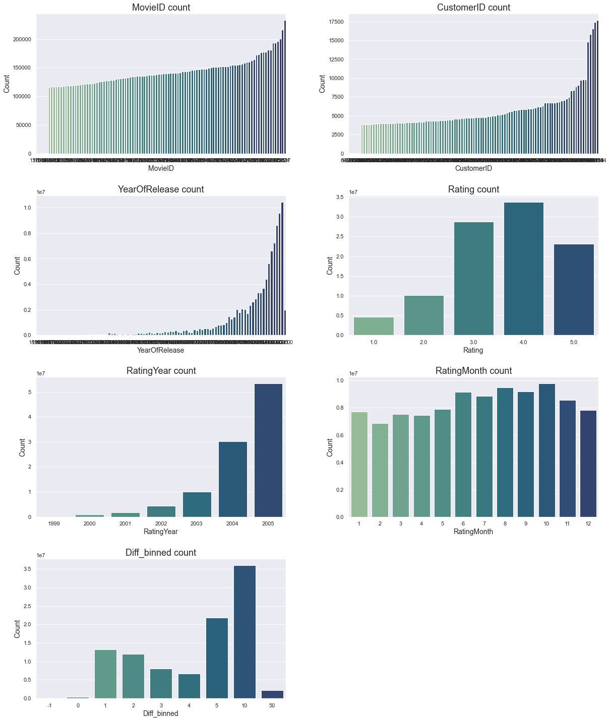
Among other things, we learn the following from above plot:

• MovieID and CustomerID counts are highly skewed with some movies receiving many reviews and some customers giving many reviews.
• Most movies are released recently.
• Most movies have received a 3 or 4 in rating, but there are also many 5s. 1s are the rarest.
• Most movies were rated in 2004 and 2005, with over 50% of the ratings in 2005. Given that most movies are released more recently, this makes sense.
• The summer months in general, but more specifically, August, September and October are the most popular months to rate a movie. Colder months, and February in particular, have the least. I wonder why. Can it perhaps be because more movies are released during these months, or is it because people have more time off. Or something else. The dataset doesn't include release date by month so we can't know for sure.
• Few movies are rated close to their release date (Diff_binned = 0). A lot of movies are rated the year after their release or within five years thereafter. Many movies are also rated over ten years after their release, which makes sense when we know that Netflix was first launched in 1997 - decades after many movies. The interpretation of this last plot depends of course a lot on how we binned the column before. And as previously stated, binning is something that should be experimented with for best result.

Machine Learning modelling

With a smaller dataset we would prefer to train and test many models using cross-validation. However, with over 100 million ratings, we can consider the data to be more than large enough for a more traditional train / test split. 80% of the data will be dedicated for training the model while 20% for testing it. Providing a seed will allow us to replicate the results.

We can now specify target variable and features for modelling. Root Mean Squared Error (RMSE) will be used for evaluating the performance of the model. It also has the inherit advantage of being easy to interpret.

Get baseline results with Linear Regression

To have a baseline to compare further models with, we will train and evaluate one of the more simplistic algorithms on the data; Linear Regression using its default parameters.

Note that we do this on a smaller fraction of the data to speed things up (file part-00000*.parquet in our case, which contain around 2.5 million reviews).

Training takes less than 30s and results in a RMSE of 1.1516 on the train set and 1.1525 on the test set. The way to interpret this is that on average, the model is wrong by 1.15 rating points for each prediction it makes. There's practically no difference between the train and test sets, which means variance is low.

Note: After evaluating a model using the original CustomerID and MovieID features instead of the hashed alternatives, HashedCustomerID and HashedMovieID, I found practically no differences between the two. I will thus continue with the original features only.

Tune and Evaluate Multiple Regressors

In order to find the best model for the problem, we will experiment with several standard algorithms: Train, tune, evaluate and test Decision Trees, Random Forests, Gradient-Boosted Trees and Linear Regressors on the dataset. Each algorithms has different hyperparameters to tune which we specify in a list of dictionaries. For example, for Random Forest, we will evaluate 20, 40 and 60 number of trees (numTrees) and a max depth (maxDepth) of each tree of 3 and 5. This results in six models only for Random Forest (2x3=6). We won't dig into the details of what these hyperparameters exactly do other than mention that they can affect the final model performance quite a lot.

Lastly, we will split the training data into 75% for training and 25% for validation, keeping a slightly larger chunk for validation as the dataset is now being split up quite some times. We make sure to use all the laptop's cores (8) to speed things up. The code for these steps are shown below.

The above process terminates in around 11 minutes and yields the following results:

	RMSE train	RMSE test
DecisionTreeRegressor	1.14973	1.15098
RandomForestRegressor	1.15065	1.15171
GBTRegressor	1.14881	1.15005
LinearRegression	1.15156	1.15247

Although with a very small margin, the Gradient-Boosted Tree Regressor (GBTRegressor) is the most performant model on the test data. Let's extract the best parameters and train it on the entire dataset.

Train the Best GBTRegressor on the Full Dataset

Using the best hyperparameters from above, we can now train and test the model on all the available data.

After 1h and 25min the training terminates and we have a final score of 1.149 - on both the train and test set. It's barely better than the 1.152 baseline though, and significantly worse than the 0.8572 the team who won the challenge in 2009 got.

Let's further explore which of the features impact the model the most in making predictions.

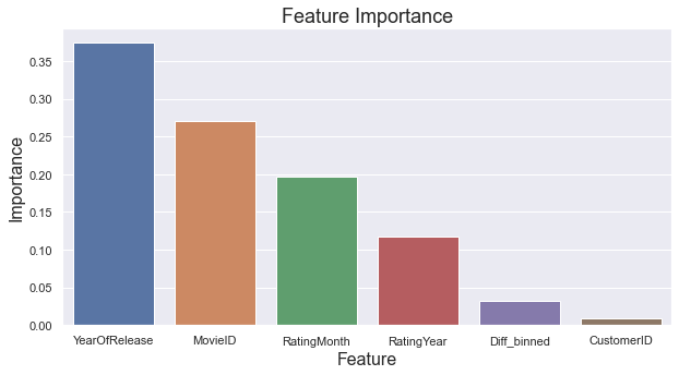
Which Features are most Important?

Tree based models return something referred to as feature importance, which can be used to better understand how the predictions are made. As displayed below, the most important features are YearOfRelease, MovieID and RatingMonth, contributing 37%, 27% and 20%, respectively. It makes sense that the movie itself (MovieID) highly impacts the model's decision. However, it's more surprising that both release year and rating month play such large roles. The difference between the release and rating year, Diff_binned contributes a meek 3% to the overall, while CustomerID contributes less than 1 percent. So much for our feature engineering efforts.

Conclusions

We've trained a few models on the 100 million ratings dataset from the Netflix challenge back in 2009 using nothing but a laptop. Although the model performance isn't as good as what was attained by the winning teams (they reportedly spent 2,000 hours during the first year of the competition), we've been successful in training a fairly large dataset locally. This in less time than what it takes to return from an outdoor exercise session. Pretty cool for just a laptop!

A final score of 1.149 RMSE (interpreted as 1.149 rating points off on each prediction, on average) was achieved while identifying YearOfRelease, MovieID and RatingMonth to be the most important features when predicting a movie's rating. This is not to say that other features wouldn't be important in making this prediction, but rather that out of the features we used, these are the most important.

We only briefly covered feature engineering - the process of creating new features out of current or external data - but this is often an incredibly important aspect in machine learning with significant predictive benefits. Examples of engineered features can be the average rating per movie or year, or count/average of ratings per day and movie, number of days since a customer's first rating, and many more.

Lastly, I should mention that although it was possible to train a model on a laptop we would benefit greatly by using a cloud service such as GCP or AWS. The cost of running an analysis of this size is so low these days that it's often a no-brainer to use them. Also, thanks to Jared Pollack from our discussion about it some time ago which inspired me to take a look at the dataset